Excel VBA – Get the Size of a Range

Sometimes the size of the selected range is determined dynamically. I need to check the number of rows and columns in the selected range. The following macro can do the work.

 Sub SizeOfRange()

    Dim Rng As Range

    Dim RowCount, ColCount As Integer

    '-----The size of range is determined dynamically.

    Set Rng = ActiveSheet.Range(Cells(6, 3), Cells(Cells(6, _ 3).End(xlDown).Row, Cells(6, 3).End(xlToRight).Column))

    '---- The number of rows and columns of the range

    RowCount = Rng.Rows.Count

    ColCount = Rng.Columns.Count

    MsgBox "The number of row is " & RowCount

    MsgBox "The number of Column is " & ColCount

End Sub

© Copyright Exceltipsandkeys All Rights Reserved.

Excel VBA – Copy Filtered data using Autofilter in VBA into Array

Autofilter commend can quickly filter out the information satisfied the criteria. Is there some way to select the data that are found after an autofilter using VBA?

Here, I prefer to transfer the data to an array so that I can use them in other calculation.

 Step 1, Autofilter the range

Step 2, Copy the visible cells into the array for further use

The key commend I used here is that If Rng(i,1).Rows.Hidden = False Then Copy the data into the destination array which is transferred into the main sub later.

Sub main()

    Dim FiltResult() As Variant

    Dim Filtersheet As Worksheet

    Dim FiltRange As Range

    Dim FiltField As Integer

    Dim FiltCrit As Variant

    Set Filtersheet = sheets("Sheet1")

    Set FiltRange = Filtersheet.Range("C6:F7380")

    FiltField = 1

    FiltCrit = 910

    FiltResult = Copyfilter(Filtersheet, FiltRange, FiltField, FiltCrit)

    '''''

    ''''Codes related with the filtered result

    ''''

End Sub

Function Copyfilter(Sht As Worksheet, Rng As Range, FField As Integer, Crit As Variant)

         Dim Arr() As Variant

           Sht.Select

         With Sht

          'Remove any existing filters

 Rng.AutoFilter

           RowCount = Rng.Rows.Count

           ColCount = Rng.Columns.Count

           Count = 1

           ReDim Arr(1 To RowCount, 1 To ColCount)

           Rng.AutoFilter Field:=FField, Criteria1:=Crit

            '------Copy the data to array for future use

           For i = 2 To RowCount

                If Rng(i, 1).Rows.Hidden = False Then

                   For j = 1 To ColCount

                   Arr(Count, j) = Rng(i, j).Value

                   Next j

                   Count = Count + 1

                 End If

            Next i

          'Remove the filter

           Rng.AutoFilter

        End With

        '----Transfer the data to the main sub

        Copyfilter = Arr

End Function

                                                                                 © Copyright Exceltipsandkeys All Rights Reserved.

Excel VBA – Select Filtered data using Autofilter in VBA via a Temporary Sheet

Autofilter commend can quickly filter out the information satisfied the criteria. Is there some way to select the data that are found after an autofilter using VBA?

Here is one method I use.

Step 1, Add a temporary sheet

Step 2, Copy and paste the filtered result to the temporary sheet
Step 3, Manipulate the data
Step 4, Delete the temporary sheet
 

The key commend I used here is .SpecialCells(xlCellTypeVisible), which allow to copy only the filtered results.

Sub main()

    Dim FiltResult As String

    Dim Filtersheet As Worksheet

    Dim FiltRange As Range

    Dim FiltField As Integer

    Dim FiltCrit As Variant

    Set Filtersheet = sheets("Sheet1")

    '---The targeted range object

    Set FiltRange = Filtersheet.Range("C6:F7000")

    FiltField = 1

    FiltCrit = 900

    FiltResult = Copyfilter(Filtersheet, FiltRange, FiltField, FiltCrit)

    '''''

    ''''Codes related with the filtered result

    ''''

    '------Delete the temporary sheet

    sheets(FiltResult).Delete

End Sub

Function Copyfilter(Sht As Worksheet, Rng As Range, FField As Integer, Crit As Variant)

        Dim Sh1 As Worksheet

        '------Add a temporary sheet to save the filtered result

        Set Sh1 = Worksheets.Add

        '------Transfer the name of the temporary Sheet to the main program

        Copyfilter = Sh1.Name

        Sht.Select

        With Sht

            'Remove the previous filter if any      

            Rng.AutoFilter 

            Rng.AutoFilter Field:=FField, Criteria1:=Crit

            '----Copy the data to temporary sheet for future use

            Rng.SpecialCells(xlCellTypeVisible).Copy Destination:=Sh1.Range("A1")

            'Remove the filter

            Rng.AutoFilter Field:=FField

        End With

End Function

© Copyright Exceltipsandkeys All Rights Reserved.

Excel VBA – Use Run time error to program

It is annoying to see the error messages when the program runs. Figuring out the cause of the error and fixing them may take even longer time than coding.

One of the errors is the run time error which occurs when VBA cannot correctly execute a program statement. This is the error I sometimes use to fulfill my program goal.

 For example, one of the typical run time errors is accessing a non-existent worksheet. I used this error message to help me determine whether the worksheet exists, otherwise build a new one.

Sub main()

Dim Filename As String

Filename = "NewSheet"

Call NewTab(Filename)

End Sub

Function MakeNewTab(Filename As String)

    On Error Resume Next

    Sheets(Filename).Select

    If Err.Number <> 0 Then

      Sheets.Add.Name = Filename

    End If

End Function

Another example is to use Error message to find the missing records.

Sub SearchRecord()

    Dim Fingwhat As String

    Dim Rng As Range

    Dim FindResult As Range

    Findwhat = 91          '''''' The record which is searched

    Set Rng = Range("C8:C1000")          ''''The searching Range

    Set FindResult = Rng.Find(Findwhat, LookIn:=xlValues)

    On Error Resume Next                 ''''The search result

    c = FindResult.Address

    If Err.Number <> 0 Then MsgBox "Can Not Find " & Findwhat

End Sub

                                © Copyright Exceltipsandkeys All Rights Reserved.

Excel VBA – Dynamic arrays and ReDim make the code flexible

When I code in VBA, it is very rare that I will deal with a fixed number of the objects. I like to use dynamic arrays and then use ReDim to resize the array to the necessary dimensions, which makes core more flexible and adoptable in the different place.

For example,

  Dim PmtStream() As Variant

    '----we read the date from Excel sheet to PmtStream. The count variable is used to count the number of values read in.

    TotalCount = WorksheetFunction.CountIf(Range("F2:F100"), ">0")

    '-----ReDim PmtStream to the size which is needed.

    ReDim PmtStream(1 To TotalCount)

    Count = 1

    For i = 2 To 100

         If Cells(6, i).Value > 0 Then

         PmtStream(Count) = Cells(6, i).Value

        Count = Count + 1

        End If

     Next i

This is the good way to control the size of the array.

© Copyright Exceltipsandkeys All Rights Reserved.

Excel and Excel VBA - Convert column letter to number

The columns of the excel sheet are labeled as ‘A’, ‘B,’ ‘C’…. It looks straightforward but it gives the difficult when I did VBA programming.

What is the corresponding number to the column K?

1) Count by figure.

2) In Cell A1, type in =1

             In Cell B1, type in  “=A1+1”
             Then, drag the formula from Cell B1 to Cell K1

3) In Cell A1, type in  =CODE("K")-64

The second question, what is the corresponding number to the column BK?

1) Count by figure. (I do not think it is a good idea)

2) In Cell A1, type in =1
             In Cell B1, type in  “=A1+1”
             Then, drag the formula from Cell B1 to Cell BK1 (It is not a good idea neither)

3) In Cell A1, type in  =(CODE("B")-64 )*26+(CODE("K")-64 )

 Therefore, you can see the method 1 and 2 are not bad for the first couple of excel columns but it is not a good idea when number of columns is increased.

Method 3 is a good idea.

The method 4 is using VBA code. I prefer this.

Sub ColumnLetterToNumber()

Dim InputLetter As String
Dim OutputNumber As Integer
Dim Leng As Integer
Dim i As Integer

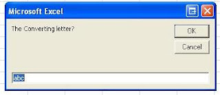
InputLetter = InputBox("The Converting letter?")  ' Input the Column Letter
Leng = Len(InputLetter)
OutputNumber = 0

For i = 1 To Leng

   OutputNumber = (Asc(UCase(Mid(InputLetter, i, 1))) - 64) + OutputNumber * 26
Next i

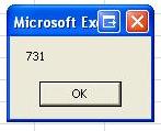
MsgBox OutputNumber   'Output the corresponding number
 

End Sub

Using the above code, I can quickly find the number I need. And both lower case and upper case letter give the same result.

For example,

Input letter = “abc”

Output number = 731

                                                                                        © Copyright Exceltipsandkeys All Rights Reserved.

Excel – Insert Date and Filename for Future Reference

Do you have the experience you have the hard time to find the original Excel spreadsheet they use when you review your coworker’s print out work? Or there are several files having similar name and you could not figure out which one is the right one.

It is very important to have date and filename showing in the print out version.

One thing we can do using Page Setup in the Print Preview. Either Custom Header or Custom Footer allow us to insert time and file path, file name and sheet name.

However, I prefer to use the formula.

NOW() displays the current date and time. The value updates when the excel sheet is reopened.

CELL("filename") display the full path including file path, file name and sheet name.

 Nearly all of my work has these two formulas in it.

When we review the printed out in the file, there are no problem to know when the work is done and where it is saved.

One more handy thing to do is to insert the current date so we know when is the last time the excel sheet is modified.

In the cell you want to save the date, press Ctrl + ;

© Copyright Exceltipsandkeys All Rights Reserved.