Excel VBA – Dynamic arrays and ReDim make the code flexible

When I code in VBA, it is very rare that I will deal with a fixed number of the objects. I like to use dynamic arrays and then use ReDim to resize the array to the necessary dimensions, which makes core more flexible and adoptable in the different place.

For example,

  Dim PmtStream() As Variant

    '----we read the date from Excel sheet to PmtStream. The count variable is used to count the number of values read in.

    TotalCount = WorksheetFunction.CountIf(Range("F2:F100"), ">0")

    '-----ReDim PmtStream to the size which is needed.

    ReDim PmtStream(1 To TotalCount)

    Count = 1

    For i = 2 To 100

         If Cells(6, i).Value > 0 Then

         PmtStream(Count) = Cells(6, i).Value

        Count = Count + 1

        End If

     Next i

This is the good way to control the size of the array.

© Copyright Exceltipsandkeys All Rights Reserved.

Excel and Excel VBA - Convert column letter to number

The columns of the excel sheet are labeled as ‘A’, ‘B,’ ‘C’…. It looks straightforward but it gives the difficult when I did VBA programming.

What is the corresponding number to the column K?

1) Count by figure.

2) In Cell A1, type in =1

             In Cell B1, type in  “=A1+1”
             Then, drag the formula from Cell B1 to Cell K1

3) In Cell A1, type in  =CODE("K")-64

The second question, what is the corresponding number to the column BK?

1) Count by figure. (I do not think it is a good idea)

2) In Cell A1, type in =1
             In Cell B1, type in  “=A1+1”
             Then, drag the formula from Cell B1 to Cell BK1 (It is not a good idea neither)

3) In Cell A1, type in  =(CODE("B")-64 )*26+(CODE("K")-64 )

 Therefore, you can see the method 1 and 2 are not bad for the first couple of excel columns but it is not a good idea when number of columns is increased.

Method 3 is a good idea.

The method 4 is using VBA code. I prefer this.

Sub ColumnLetterToNumber()

Dim InputLetter As String
Dim OutputNumber As Integer
Dim Leng As Integer
Dim i As Integer

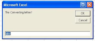
InputLetter = InputBox("The Converting letter?")  ' Input the Column Letter
Leng = Len(InputLetter)
OutputNumber = 0

For i = 1 To Leng

   OutputNumber = (Asc(UCase(Mid(InputLetter, i, 1))) - 64) + OutputNumber * 26
Next i

MsgBox OutputNumber   'Output the corresponding number
 

End Sub

Using the above code, I can quickly find the number I need. And both lower case and upper case letter give the same result.

For example,

Input letter = “abc”

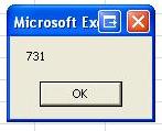
Output number = 731

                                                                                        © Copyright Exceltipsandkeys All Rights Reserved.

Excel – Insert Date and Filename for Future Reference

Do you have the experience you have the hard time to find the original Excel spreadsheet they use when you review your coworker’s print out work? Or there are several files having similar name and you could not figure out which one is the right one.

It is very important to have date and filename showing in the print out version.

One thing we can do using Page Setup in the Print Preview. Either Custom Header or Custom Footer allow us to insert time and file path, file name and sheet name.

However, I prefer to use the formula.

NOW() displays the current date and time. The value updates when the excel sheet is reopened.

CELL("filename") display the full path including file path, file name and sheet name.

 Nearly all of my work has these two formulas in it.

When we review the printed out in the file, there are no problem to know when the work is done and where it is saved.

One more handy thing to do is to insert the current date so we know when is the last time the excel sheet is modified.

In the cell you want to save the date, press Ctrl + ;

© Copyright Exceltipsandkeys All Rights Reserved.

Excel - Convert column letter to number using COLUMN()

Every day, I find some new things or have new idea in the Excel. I suddenly figure it out a simple way to convert column letter to numbers. By modifying it, I can also quickly determine the column index number used in the VLOOKUP() function.

It is COLUMN() function.

For example,

What is the column number for column AB?

In cell A1, type in the formula =COLUMN(AB1).

The result is 28.

What is the corresponding column numbers for column BA to column BE?

In cell A1, type in the formula =COLUMN(BA1). Then drag the formula from A1 to E1.

The result is 53,54,55,56,57.

What is the column index number assuming a table array is from column G to column BA and the target column is Column AY?

In cell A1, type in the formula =COLUMN(AY1)-COLUMN(G1)+1.

The result is 45.

   

                                                                                © Copyright Exceltipsandkeys All Rights Reserved.

Excel – ADDRESS() Convert number to the column letter

I figure out an easy way to find the corresponding column from the column number.

It is ADDRESS(row_number,column_number, ) Function.

For example,

Which column is column 20?

In cell A1, type in formula =ADDRESS(1,20)

The result is $T$1.

The answer is column T.

It can also be used to quickly determine the target column (index column) in the VLOOKUP() function with the help of COLUMN() function.

ADDRESS(1,COLUMN(the first cell of the table array)+column _index number-1)

For example,

Which column we look up in the formula VLOOKUP(D14,K14:BP21,21,0)?

In cell A1, type in formula =ADDRESS(1,COLUMN(K14)+21-1)

The result is $AE$1.

The answer is column AE

Excel - Find the last row or column used in the sheet

Sometime we wrote VBA code to find the last used cells in the sheet.

Sub LastCellInSheet()

Dim i, j, RowNo, ColumnNo As Integer

'i, j decide the column or row you are interested in

i = 1

j = 1

RowNo = Cells(Rows.Count, j).End(xlUp).Row

ColumnNo = Cells(i, Columns.Count).End(xlToLeft).Column

  

End Sub

For example,

The result from running the above code is

RowNo = 10

ColumnNo = 3

However, if there is the data in the last column (Column XFD for excel 2007) or in the last row (Row 1048576 for excel 2007) , the code would give us the wrong information. The code would not count the last column and lost row.

It would not be a big issue because there is no record in the last column or last row in most of the cases. However, If you want to make sure the code is always working, we can modify the above code.

Dim i, j, RowNo, ColumnNo As Integer

'i, j decide the column or row you are interested in

i = 1

j = 1

If Cells(Rows.Count, j) <> "" Then RowNo = Rows.Count Else RowNo = Cells(Rows.Count, j).End(xlUp).Row

If Cells(i, Columns.Count) <> "" Then ColumnNo = Columns.Count Else ColumnNo = Cells(i, Columns.Count).End(xlToLeft).Column

© Copyright Exceltipsandkeys All Rights Reserved.

Excel - Find the last row or column in the Data Range

Sometime we wrote VBA code to find the last cells in a data range.

If there is no blank in the middle of the data range, the following code can be used.

    Sub LastCellInRange()

    RowNo = Range("A1").End(xlDown).Row

    ColumnNo = Range("A1").End(xlToRight).Column

    End Sub

However, if there is the data range contains only one data, the code would give us the wrong information.

For example,

The result from running the above code is

RowNo=1048576

ColumnNo=16384

By modifying the above code, we can get the right answer.

Sub LastCellInRange()

Dim i, j, RowNo, ColumnNo As Integer

'i,j decide the location of the first cell in the range

i = 1

j = 1

If Cells(i + 1, j) <> "" Then RowNo = Cells(i, j).End(xlDown).Row Else RowNo = i

If Cells(i, j + 1) <> "" Then ColumnNo = Cells(i, j).End(xlToRight).Column Else ColumnNo = j

 

End Sub

The result from running the above code is

RowNo=1

ColumnNo=1

© Copyright Exceltipsandkeys All Rights Reserved.

EXCEL - SUBTOTAL(function_num,ref)

Subtotal function can use to calculate the different totals such as Sum, Average and etc. For a long time, I could not understand why people bother to use subtotal function instead of corresponding function, such as Subtotal(1,ref)=average(ref). We have to remember or spend a minute to figure out which number we use.

Once, I build a report. The target audience wants to see the total value based on the criteria they filter the data. Then, I realized the power of SUBTOTAL Function.

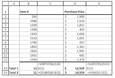
For example, we want to calculate the total number of the items we bought and total values of the price we paid.

The SUBTOTAL() and COUNT() and SUM() functions gave us the same results.

However, if we filter the data and use the criteria (purchase price > $1,000), you can that the total values are different. SUBTOTAL() includes only the values which satisfy the criteria but COUNT() or SUM() include all the values.

© Copyright Exceltipsandkeys All Rights Reserved.

EXCEL - Count the number of rows and columns in the Sheet

When we use the Excel to record, I am curious about how many records I can put into the spreadsheet.

The following Macro can do the job.

Sub RowandColumnCount()

MsgBox Rows.Count

MsgBox Columns.Count

End Sub

My Excel version is Excel 2007.

The outputs are 1,048,576 and 16,384.

I can have 1,048,576 row of records and 16,384 column of records.

© Copyright Exceltipsandkeys All Rights Reserved.

Create the description of the income or outcome stream.

Sometimes, a descriptions of the payment stream needs to be generated in the contracts or other legal documents.

For example,
We have the following payment stream in the excel.

We would like to generate the payment description as the following;

3 Monthly payments of $ 76.83 per month, beginning November 6, 2018 through and including January 6, 2019;  12 Monthly payments of $ 300.00 per month, beginning February 6, 2019 through and including January 6, 2020;  12 Monthly payments of $ 500.00 per month, beginning February 6, 2020 through and including January 6, 2021;  12 Monthly payments of $ 656.00 per month, beginning February 6, 2021 through and including January 6, 2022; 1 payment in the amount of $ 5,000.00 due on February 6, 2021;

You can type in the description. It would not take long time to do one. However, it would be a terrible task if we have to do it more than 10 times.

One method is to use the formula

Step 1: In the Cell I5, Formula = IF(E5>1,CONCATENATE(E5," monthly payments of $",TEXT(D5,"#,###.00")," per month, beginning ",TEXT(C5,"mmmm d,yyyy")," through and including ",TEXT(C5,"mmmm d,yyyy")),CONCATENATE("1 payment in the amount of $ ",TEXT(D5,"#,###.00")," due on ",TEXT(C5,"mmmm d,yyyy")))

Step 2: Copy the formula to from Cell I6 to I9.

Step 3: In Cell J6, Formula= I5&"; "&I6

Step 4: Copy the formula to from Cell J7 to J9.

Step 5: J9 is the final description we need. It can be copied to the word document.

Another method is to use VBA Code.

Sub Description()

Dim PStream As String

Dim i As Integer

Set wk1 = ActiveSheet

PStream = ""

wk1.Range("H1").ClearContents

i = 12

Do While wk1.Cells(i, 1) <> ""

   

    If wk1.Cells(i, 5).Value = 1 Then

        Des = "1 payment of $" & Format(wk1.Cells(i, 4), "#,##0.00") _

        & " due on " & Format(wk1.Cells(i, 3), "mmmm d, yyyy") & "; "

    Else

        Des = Format(wk1.Cells(i, 5), "#,##0") & " " & "monthly payments of $" & Format(wk1.Cells(i, 4), "#,##0.00") _

        & " per month, beginning " & Format(wk1.Cells(i, 3), "mmmm d, yyyy") & " through and including " & Format(wk1.Cells(i, 7), "mmmm d, yyyy") & "; "

    End If

   

    i = i + 1

    PStream = PStream & Des

Loop

wk1.Range("H1") = PStream

End Sub

Calculate Age in Excel (2) - the age at the nearest birthday

Several functions in EXCEL can be used to determine the age such as, DATEDIF(), YEARFRAC().

Which one should be applied depends on the definition of the age.

The age is defined as age at nearest birthday.

·       Method 1,    DATEDIF(DATE1,DATE2,”m”) Combined with ROUND()

For example,

DOB (Date of Birth)                 5/20/1976

DOT (Date of Target)               11/20/2012

AGE at DOT                                                  37

In Cell B1, Type in 5/20/1976

In Cell B2, Type in 11/20/2012

In Cell B3, Formula= =ROUND(DATEDIF(B1,B2,"m")/12,0)

Thus, The Formula is ROUND(DATEDIF(DOB, DOT, ”m”)/12,0)

·       Method 2, YEARFRAC(DATE1,DATE2,0) Combined with INT()

In Cell B1, Type in 5/20/1976

In Cell B2, Type in 11/20/2012

In Cell B3, Formula= =INT(YEARFRAC(B1,B2,0)+0.5)

Thus, The Formula is INT(YEARFRAC(DOB, DOT, 0)+0.5)

© Copyright Exceltipsandkeys All Rights Reserved.